%matplotlib inline
%config InlineBackend.figure_format = 'retina'
import matplotlib.pyplot as plt
import numpy as np
from matplotlib.colors import Normalize

Simple Usage

If you only need the linear power spectrum, only the basic class CBaseEmulator is needed.

import sys
sys.path.append('../')
from CEmulator.Emulator import CBaseEmulator

##### import the emulator for the original cosmology [only one single massive neutrino]
csstemu = CBaseEmulator(verbose=True, neutrino_mass_split='single')
klists  = np.logspace(-4.5, 2, 500)
zlists  = np.array([0.0, 1.0, 2.0, 3.0])

Loading the PkcbLin emulator...
Using 513 training samples.
Loading the PknnLin emulator...
Using 512 training samples [remove c0001 (no massive neutrino)].
The neutrino mass is treated as a single massive component.

%%time
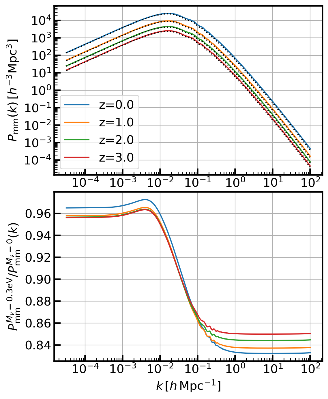
csstemu.set_cosmos(As=2.1e-9, mnu=0.0)
pklin0 = csstemu.get_pklin(z=zlists, k=klists, Pcb=False)
csstemu.set_cosmos(As=2.1e-9, mnu=0.3)
pklin1 = csstemu.get_pklin(z=zlists, k=klists, Pcb=False)

CPU times: user 10 ms, sys: 225 µs, total: 10.2 ms
Wall time: 9.5 ms

with plt.style.context('article'):
    gridplt = plt.GridSpec(2, 1, hspace=0.1)
    plt.figure(figsize=(6, 8))
    plt.subplot(gridplt[0])
    for ii in range(len(zlists)):
        plt.plot(klists, pklin0[ii], label='z={}'.format(zlists[ii]))
        plt.plot(klists, pklin1[ii], 'k:')
    plt.legend()
    plt.xscale('log')
    plt.yscale('log')
    plt.ylabel(r'$P_{\rm mm}(k)\,[h^{-3}{\rm Mpc}^3]$')
    plt.subplot(gridplt[1])
    for ii in range(len(zlists)):
        plt.plot(klists, pklin1[ii]/pklin0[ii], label='z={}'.format(zlists[ii]))
    plt.ylabel(r'$P^{M_\nu=0.3 \mathrm{eV}}_{\rm mm}/P^{M_\nu=0}_{\rm mm}(k)$')
    plt.xlabel(r'$k\,[h\,{\rm Mpc}^{-1}]$')
    plt.xscale('log')

Compare with CLASS and CAMB

%%time
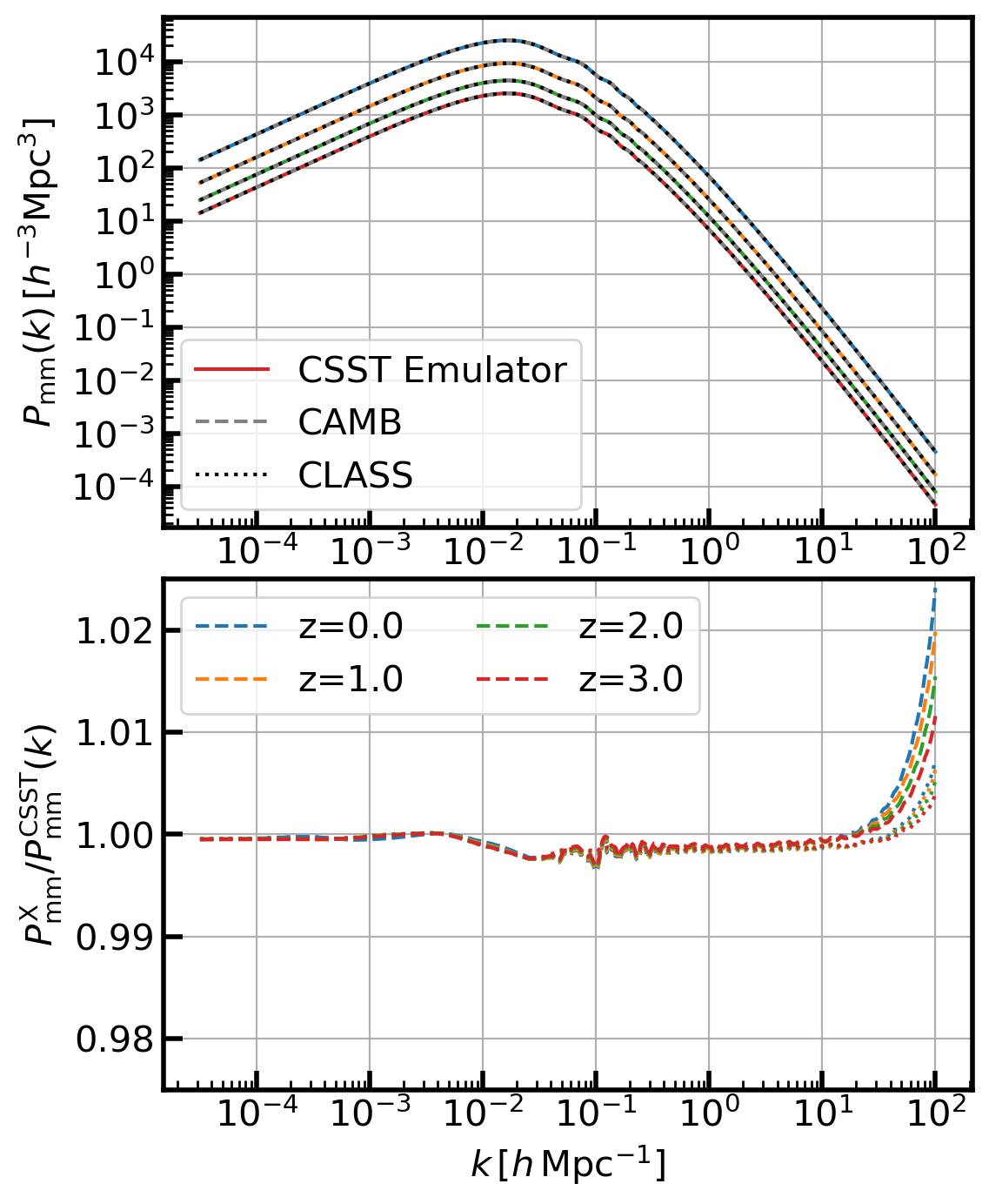
csstemu.set_cosmos(As=2.1e-9, mnu=0.0)
pkmmce = csstemu.get_pklin(z=zlists, k=klists, Pcb=False)

CPU times: user 4.48 ms, sys: 1.93 ms, total: 6.42 ms
Wall time: 5.7 ms

%%time
cosmo_class = csstemu.get_cosmo_class(z=zlists, kmax=100.0, non_linear='HMCODE')
pkmmcl = np.zeros((len(zlists), len(klists)))
h0 = csstemu.Cosmo.h0
for iz in range(len(zlists)):
    pkmmcl[iz] = np.array([cosmo_class.pk_lin(z=zlists[iz], k=ik*h0)*h0*h0*h0 for ik in klists])

CPU times: user 8.08 s, sys: 36.5 ms, total: 8.12 s
Wall time: 8.13 s

%%time
camb_results = csstemu.get_camb_results(z=zlists, kmax=100.0, non_linear='mead2020')
pkmmca = camb_results.get_matter_power_interpolator(nonlinear=False,
                                                    var1='delta_tot', var2='delta_tot',
                                                    hubble_units=True, k_hunit=True).P(z=zlists, kh=klists)

CPU times: user 6.3 s, sys: 26.7 ms, total: 6.33 s
Wall time: 6.34 s

colors = ['C0', 'C1', 'C2', 'C3']
with plt.style.context('article'):
    gridplt = plt.GridSpec(2, 1, hspace=0.1)
    plt.figure(figsize=(6, 8))
    plt.subplot(gridplt[0])
    for ii in range(len(zlists)):
        l0, = plt.plot(klists, pkmmce[ii], color=colors[ii])
        l1, = plt.plot(klists, pkmmca[ii], color='gray', ls='--')
        l2, = plt.plot(klists, pkmmcl[ii], color='k', ls=':')
    leg2 = plt.legend([l0, l1, l2], ['CSST Emulator', 'CAMB', 'CLASS'], loc='lower left')
    plt.xscale('log')
    plt.yscale('log')
    plt.ylabel(r'$P_{\rm mm}(k)\,[h^{-3}{\rm Mpc}^3]$')
    plt.subplot(gridplt[1])
    for ii in range(len(zlists)):
        plt.plot(klists, pkmmca[ii]/pkmmce[ii], '--', color=colors[ii], label='z={}'.format(zlists[ii]))
        plt.plot(klists, pkmmcl[ii]/pkmmce[ii], ':', color=colors[ii])
    plt.legend(ncol=2)
    plt.ylabel(r'$P^{\rm X}_{\rm mm}/P^{\rm CSST}_{\rm mm}(k)$')
    plt.xlabel(r'$k\,[h\,{\rm Mpc}^{-1}]$')
    plt.xscale('log')
    plt.ylim(0.975, 1.025)